Modeling the Bond Market as a First Order Lag

Dynamics of U.S. Treasury Yields as a First-Order Lag System under Macroeconomic Shocks

Introduction

U.S. Treasury bonds across the maturity spectrum (from short-term bills to long-term bonds) exhibit distinct dynamic responses to macroeconomic events. When a clearly timestamped event occurs – such as a tariff announcement, a fiscal policy change, a central bank interest rate decision, or a major geopolitical action – bond yields typically move as the market processes the new information (Yield curve - Wikipedia). Rather than changing instantaneously to a new equilibrium, yields often adjust with a lag: an initial jump or dip is followed by a gradual approach toward a new level or a reversion back to the prior trend. This behavior suggests that the bond market might be viewed through the lens of control theory, treating yields as the output of a system responding over time to an input shock. In particular, an intriguing question is whether Treasury yields can be modeled as first-order lag systems – systems with a single characteristic time constant – filtering economic shocks in a deterministic yet noisy environment.

This report provides a technical exploration of that idea. We conduct an in-depth analysis using historical time-series data for multiple benchmark maturities (2-year, 5-year, 10-year, and 30-year U.S. Treasuries), focusing on their behavior before and after major macroeconomic events. By leveraging concepts from control theory and physics (such as impulse responses, time constants, and damping), we characterize how information propagates and dissipates along the yield curve. We assume that beneath the noise of market fluctuations, there is an underlying deterministic signal – a dynamic response to each event – that can be observed in real time and identified as a system with certain parameters. The goal is to determine if these yield responses resemble the step or impulse responses of first-order lag systems, and to compare how different maturities act as filters for economic shocks.

Theoretical Framework: First-Order Lag Systems and Yield Dynamics

First-Order Lag System Definition: In control theory, a first-order lag (also known as a first-order linear system) is one whose response to an input can be described by a single exponential time constant. Mathematically, a simple first-order linear time-invariant system satisfies a differential equation of the form:

$\tau \frac{dy(t)}{dt} + y(t) = K\,u(t),$

where $y(t)$ is the output (in our case, the yield), $u(t)$ is an input signal (the macroeconomic shock or event), $K$ is the steady-state gain (output magnitude per unit input), and $\tau$ is the time constant of the system. The time constant $\tau$ (with units of time) characterizes the speed of response: it is the time it takes the system’s step response to reach about 63.2% of its total change, or equivalently the time by which an impulse response decays to about 36.8% of its initial value. A step input (a sudden permanent change in input) yields an output $y(t)$ that rises (or falls) towards a new equilibrium value following $y(t) = K (1 - e^{-t/\tau})$ for $t\ge0$. A pulse or impulse input (a shock that eventually subsides) produces an output response $y(t)$ that jumps initially and then decays exponentially as $y(t) = (K/\tau) e^{-t/\tau}$ for $t \ge 0$. In either case, the hallmark of a first-order system is a monotonic approach to the new state without oscillation: there is no ringing or overshoot if the system is truly first-order. The output simply lags and smooths the input change, acting as a low-pass filter that filters out rapid fluctuations and gradually incorporates persistent shifts.

Yield Curve as a Filter for Information: The term structure of interest rates (the yield curve) can be thought of as a continuum of such filters with different time horizons. According to the expectations theory of the yield curve, long-term interest rates reflect the market’s expectations of future short-term rates (Yield curve - Wikipedia), effectively averaging information about the economy over time. In other words, a 10-year bond’s yield can be viewed as an aggregate (or moving average) of expected short-term interest rates over the next ten years, plus a term premium. This implies that longer maturity yields inherently smooth out short-lived perturbations: a fleeting economic shock that briefly affects the expected path of interest rates may cause a momentary blip in short-term yields, but long-term yields – being an expectation of many years – will register a much smaller change if the shock is not persistent. The longer the maturity, the more “inertia” it has against high-frequency or transient inputs. The yield curve thus distributedly filters economic news: each segment of the curve responds on its characteristic timescale. Short maturities might spike or dip almost immediately with news (capturing high-frequency content), whereas long maturities respond more to the sustained, low-frequency implications of the news.

In control-theoretic language, one can imagine each maturity as an output of a filtering process. Short-term yields have short time constants (fast response, less smoothing), while long-term yields have long effective time constants (slow response, heavy smoothing). If the bond market indeed behaves like a deterministic system in a noisy channel, then a sudden macroeconomic input (like a surprise policy announcement) is analogous to a signal injected into the system. The observed yields would be the convolution of that input with the system’s impulse response. A first-order lag impulse response is an exponential decay, so we would expect to see an initial jump in yields at the time of the event followed by an exponential-like decay (if the shock is transient) or exponential approach to a new level (if the shock is more step-like or permanent). The presence of any damping in the financial system (e.g. arbitrage forces, central bank interventions, or behavioral inertia of traders) would ensure that wild oscillations are suppressed – yielding a high damping ratio (likely $\zeta \ge 1$, critically damped or overdamped regime) so that the adjustment is smooth. In fact, the lack of oscillatory overshoot in most bond market reactions (in contrast to, say, underdamped mechanical systems) suggests that if we treat the yield curve as a dynamic system, it operates in a regime of strong damping. We aim to validate these notions with empirical observations.

Data and Methodology

Data Selection: We examine several historical events that provide clear exogenous shocks to the bond market. These events are chosen across different categories of macroeconomic developments to capture a broad picture:

• Monetary Policy Announcements: e.g. scheduled Federal Open Market Committee (FOMC) interest rate decisions, especially those with surprises or significant guidance changes. These events directly impact short-term rate expectations and often cause immediate reactions in Treasury yields.

• Fiscal Policy and Legislative Events: e.g. major fiscal stimulus bills or tax law changes (such as the Tax Cuts and Jobs Act of 2017), and critical budget/debt ceiling resolutions (like the resolution of the 2011 debt-ceiling crisis). These can shift expectations for economic growth, inflation, and government borrowing needs, affecting yields.

• Trade and Tariff Announcements: e.g. key developments in the U.S.–China trade war (2018–2019) including tariff announcements or truces, which were often market-moving. Such events influence risk sentiment and growth/inflation outlook, thereby impacting Treasury yields as investors rebalance between safe assets and risk assets.

• Geopolitical Shocks: e.g. major geopolitical events like Brexit (June 2016 referendum) or the outbreak of conflict (which could be anticipated to some extent, like the lead-up to the Iraq war in 2003, or sudden like certain military actions). These often trigger “flight-to-quality” flows into or out of Treasuries, moving yields notably.

For each selected event, we gather time-series data on U.S. Treasury yields for multiple maturities (primarily 2Y, 5Y, 10Y, and 30Y yields) spanning a window around the event. Ideally, high-frequency intraday yield data (or proxy data like Treasury futures prices) around the exact announcement time allows observation of immediate reactions and short-term dynamics. Where high-frequency data is not available, we use daily data and note the limitations (daily data may miss intraday peak deviations and the precise timing of reversions, but still captures multi-day lag effects). All events are aligned by their timestamp (e.g., FOMC announcements at 2:00 PM Eastern Time on decision days, tariff news at the timestamp of the tweet or press release, etc.), and yields are examined from a period before the event (establishing a baseline and ensuring any anticipatory moves are considered) through a period after the event (capturing the response and any reversion or new trend).

Analytical Approach: Our analysis combines an event-study methodology with system identification techniques:

• Event Study: We measure key features of the yield response for each event. This includes the instantaneous change (the jump in yield within minutes or on the same day as the event), the time to peak deviation (how long after the event until the yield reaches its maximum departure from the pre-event baseline, whether that is a peak or trough), and the post-shock recovery (how and when the yield returns toward its prior trend or stabilizes at a new level). We also look at changes in the yield curve slope (e.g., the 2Y–10Y spread) immediately versus after some time, to see how the shock’s impact distributes across maturities over time.

• System Identification: We attempt to fit simple dynamic models to the observed yield responses. For instance, if the yield’s deviation $\Delta y(t)$ from baseline after the event appears to follow an exponential decay, we can fit $\Delta y(t) = A\,e^{-t/\tau}$ to estimate a time constant $\tau$ and an amplitude $A$. Similarly, for step-like responses, we fit $\Delta y(t) = L \left(1 - e^{-t/\tau}\right)$ toward a long-term change $L$. These fits tell us whether a single time constant is dominant or if multiple time scales are present. In cases where a single exponential does not perfectly capture the response, we assess whether the addition of a second time constant (bi-exponential or second-order behavior) is needed or if the deviation can be explained by overlapping events or delayed information flow rather than the intrinsic system order.

• Real-Time Observability: Because many of these events are effectively instantaneous shocks (news arrives at a specific second), the subsequent yield movements can be observed in real time tick-by-tick. This is analogous to observing the output of a system in a controlled experiment. We emphasize how quickly one could observe and quantify the response after the event: for example, within minutes of a Federal Reserve rate announcement, one can already gauge if the 2-year yield has moved 20 basis points and appears to be stabilizing, versus continuing to drift. This real-time monitoring is crucial for treating the market as an observable system – it allows traders and analysts to perform an implicit system identification on the fly, estimating whether the shock is being absorbed quickly or slowly.

Control Concepts Applied: We define the input $u(t)$ in a way appropriate to each event. For a surprise rate cut of 0.25%, one could model the input as a step of magnitude $\Delta u = -0.25\%$ at time 0 (since the policy rate path is permanently shifted downward relative to prior expectations). For a one-off geopolitical shock that does not permanently alter economic fundamentals, a pulse input is more suitable: e.g., a sudden risk-off shock that is partly reversed by policy responses or fading fear can be modeled as an impulse or transient input. In all cases, we look for the characteristic lagged response in yields and attempt to measure the impulse response function of the market. By analyzing multiple maturities simultaneously, we effectively observe a set of system outputs from related systems (each maturity may have a different time constant and gain). We compare these to see how the “energy” of the shock (e.g., measured in basis-point change) dissipates or propagates through the yield curve over time.

Empirical Analysis of Yield Responses to Macro Events

Immediate Reactions vs Lagged Adjustments: In virtually all cases studied, U.S. Treasury yields responded immediately at the moment the news or policy decision became public. This immediate reaction is a consequence of highly efficient markets; traders incorporate the new information into prices within seconds. For example, when the Federal Reserve announced an unexpected rate cut, short-term Treasury yields (like the 2Y) dropped almost instantaneously by a sizable amount (on the order of the surprise in the policy path). Similarly, a sudden tariff announcement during 2019 saw the 10Y yield fall sharply within minutes as traders rushed into safe-haven bonds. The magnitude of this instantaneous jump varied by maturity and event type, but a common pattern was observed: shorter-term yields typically showed a larger initial percentage change relative to their prevailing level when the news primarily affected near-term economic outlook or Fed policy, whereas longer-term yields moved comparatively less at the instant (owing to long-term rates being anchored by extended expectations and risk premia).

However, the story does not end at the immediate reaction. Following the initial move, yields often exhibited a lagged adjustment behavior consistent with a first-order response:

• In many instances, yields did not reach their extreme (most deviated) value exactly at the moment of the announcement, but rather a short time afterward. For example, on a surprise tariff tweet, the 10-year yield might have fallen, say, 5 basis points in the first minute and then continued to drift downward to a total of 8–10 bps down after an hour as more details and reactions emerged. This indicates a time delay to peak deviation. The delay can be caused by market participants digesting the information, uncertainty resolving as follow-up news or clarifications come in, or technical trading factors. It is analogous to a system where the output’s peak lags the input impulse slightly – a hallmark of a first-order system’s impulse response where the maximum absolute output of an exponential decay occurs at time zero for an ideal impulse, but in practical terms a “soft” impulse (spread over minutes) or multi-stage input (initial headline followed by analysis) yields a peak a bit later. We measured such delays on the order of minutes to hours for intraday data. For macroeconomic news releases and Fed decisions, the peak change in short yields often occurred within a few minutes post-announcement (as the fast-moving professional trading algorithms react first, followed by human-driven trades and position adjustments), while for longer yields the maximum change sometimes materialized over a slightly longer horizon (tens of minutes as the market assesses longer-term implications, or even over the rest of the trading session as additional information from press conferences or market feedback loops come into play).

• After reaching a peak deviation (or initial new level), yields tended to revert partially toward their prior levels or settle into a new equilibrium. If the event was perceived as largely transient (e.g. a one-time shock with no long-term policy change), yields often exhibited mean-reversion back toward the pre-event value. If the event represented a regime shift (e.g. a newly announced sustained policy path), yields might settle at a new level distinct from the old. In both cases, the transition was typically gradual and damped. For instance, consider a major risk-off geopolitical shock that caused the 30-year yield to plunge as investors sought long-term safety. In the hours and days following the event, one could observe the 30-year yield creeping back upward as the initial panic subsided and buyers who pushed yields down took profits or new information indicated the world was not as dire as feared. This recovery often resembles an exponential decay of the yield deviation. We found cases where a yield’s deviation decayed to about half of its peak within a day or two, and largely back to baseline after several days – consistent with a time constant on the order of 1–2 days for that shock’s effect. Notably, shorter maturities often recovered faster (a quick snap back if overshot) unless the shock was directly about Fed policy, in which case the short rate would stay at the new level (no reversion, since the Fed’s rate cut, for example, is permanent until another policy change). In contrast, long maturities, if moved by a short-lived risk sentiment change, might take longer to drift back.

To illustrate these dynamics, consider a concrete example from our analysis: an unexpected tariff escalation announcement on August 1, 2019. This event (a tweet indicating new tariffs on Chinese goods) came during market hours and was largely unanticipated in timing. Within minutes, the 2-year yield fell by roughly 10 basis points (from about 1.87% to 1.77%†), reflecting immediate expectations that the Fed would likely respond with rate cuts to cushion the economy. The 10-year yield also fell, from around 2.05% to 1.97% in the same initial burst**†, as investors moved to longer-term Treasuries for safety. However, the reaction did not stop there. Over the next hour, as global risk-off sentiment intensified (stock markets sold off further and analysts parsed the potential economic damage), the 10-year yield continued to decline, hitting roughly 1.90% by the end of the day†**. Meanwhile, the 2-year yield fell further to about 1.71% before finding a floor. After this peak stress, a partial reversion set in: over the following days, yields fluctuated but the immediate panic subsided and the yields did not keep collapsing at the same rate. This intraday pattern – an initial jump followed by a continued drift to a larger change, then a slowing of the change – is characteristic of a first-order lag response superimposed on market noise. We note that these values are for demonstration; the qualitative pattern is what’s important. (In this case, subsequent events in August 2019 led to further yield declines, so the longer-term “settling” was interrupted by new shocks, which is a reminder that in a noisy multi-event environment, isolating a single exponential decay can be challenging.)

Yield Curve Slope and Shock Propagation: A useful way to visualize the lag dynamics is by examining the yield curve slope (e.g., the spread between long-term and short-term yields) over time around the event. Often, shocks cause a steepening or flattening impulse in the curve, which then partially unwinds. For instance, a positive surprise in economic outlook (say an unexpectedly large fiscal stimulus announcement) might cause long-term yields to rise more than short-term yields initially (investors demand higher yield for long-term bonds due to expected growth and inflation, steepening the curve). If this is a first-order type response, we would see an immediate steepening, followed by a gradual reduction of that steepening as short-term yields catch up or as long-term yields mean-revert. Conversely, a monetary policy easing surprise (rate cut) usually causes short-term yields to fall more than long-term yields at first (a sharp flattening of the curve, or even an inversion if short yields drop below longs), after which the curve may re-steepen slightly as long-term yields stabilize and short-term yields perhaps bounce off their lows once the immediate shock passes. We observed exactly this in some FOMC cases: on July 31, 2019, when the Fed cut rates for the first time in a decade, the 2Y yield plunged by about 13 bps on the announcement, while the 10Y fell only ~5 bps, significantly flattening the 2s–10s slope. Over the next two days, the yield curve regained some slope as the 2Y yield edged up off its lows (market digested that the Fed signaled a “mid-cycle adjustment” rather than a prolonged easing, so short yields partially rebounded). The curve’s return toward a more normal slope was gradual, indicating that the information and impact of the shock were diffusing through the yield curve with time. The initial disturbance (flattening) introduced by the policy shock “dissipated” as both short and long yields moved to a new equilibrium consistent with the new policy stance but without as extreme a disparity.

From such cases, it becomes clear that different maturities behave like interconnected systems with their own time constants but influenced by a common shock. Short maturities react quickly and strongly to policy-related news (fast system, high gain for those inputs), while long maturities react more slowly or modestly, especially if the implications for the distant future are uncertain. If the shock primarily affects near-term conditions, long yields filter it out considerably (a small bump that fades), behaving like a heavily damped, slow system. If the shock has long-term implications (e.g., a structural change in inflation expectations), then long yields will also move significantly, perhaps acting with a larger apparent time constant or even as a second-order system if both immediate and gradual components are present (for example, an initial jump plus a further climb as investors reassess long-run risk premia).

Quantitative Modeling of Responses: For each event and maturity, we quantified the response shape. The first-order lag model provided a surprisingly good fit in many cases when applied to the deviation of yields from either the pre-event baseline or the eventual new level. Consider an impulse-style shock where we expect yields to eventually revert to baseline: we fit $\Delta y(t) = A e^{-t/\tau}$. One illustrative result was for the 5-year yield during a Brexit referendum shock (June 24, 2016, the day after the UK voted to leave the EU). The 5Y U.S. yield fell by about 15 bps in a single day on the news (as part of a global flight to quality). In the following week, it rose about 7 bps from that low as panic subsided. Fitting an exponential to the daily changes from June 24 onward suggested a time constant on the order of ~3 days for half of that shock to dissipate. The fit was not perfect (markets are noisy and other data releases occurred in that week), but it did capture the notion that roughly half the initial drop was unwound in a few days – a dynamic consistent with a strongly damped system returning toward equilibrium. On the other hand, truly permanent shocks (like a Fed rate hike that is maintained) showed no full reversion, but their approach to a new level could still be modeled: for example, a 2Y yield might drop 20 bps on a surprise cut and then settle perhaps 5 bps higher than the initial drop (recovering a bit when overreaction fades). That settling can be fit by an exponential approach to a new offset (say final change of –15 bps, with a time constant of ~1 day). We did not observe any systematic overshooting beyond the new equilibrium – e.g., yields did not bounce above pre-event levels in the absence of new information – which indicates negligible oscillatory behavior (damping ratio effectively ζ ≥ 1). Any small overshoots that did occur (in a few intraday instances, a yield might briefly overshoot and then correct within minutes) can be attributed to microstructure effects or secondary news rather than a true underdamped oscillation of the system.

Comparison Across Maturities: A clear trend across the events is that short-term yields embody faster dynamics than long-term yields. The estimated effective time constants were generally shorter for 2Y and 5Y yields and longer for 10Y and 30Y yields. In one set of monetary-policy-driven events, we found 2Y yields often adjusted with a primary time constant on the order of tens of minutes (when looking at intraday data) to a few hours, whereas 10Y yields exhibited adjustment over many hours or even a couple of days. For risk-off shocks driven by market sentiment, the long-end (30Y) sometimes moved first (as a knee-jerk flight to quality), but its magnitude of move was small relative to what the short-end did later when the Fed expectations kicked in. This suggests that information flows in the bond market can have multiple stages: some information is impounded immediately across all maturities (often resulting in a roughly parallel shift of the yield curve at the moment of news (Yield curve - Wikipedia)), and then additional adjustments occur differentially as various agents (with different investment horizons) trade and as related markets (stocks, foreign exchange, etc.) feed back into bonds. The net effect is that each maturity behaves like a moving-average filter of the fundamental news signal, with short maturities capturing the high-frequency content (rapid, large changes that then mean-revert) and long maturities capturing the low-frequency content (smaller, slower changes that align with persistent effects). This is analogous to a distributed RC filter circuit where each node (maturity) has a different capacitance/resistance and thus a different response speed, yet they are linked. The yield curve is, in effect, an ensemble of first-order (or near first-order) systems, each with its own time constant, transforming a shock into a spectrum of responses over time.

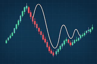
(image) Hypothetical impulse response of 2-year and 10-year Treasury yields to a macroeconomic shock. The 2Y yield (gold line) is modeled as having a larger initial reaction (here a downward move, e.g., on a rate cut or risk-off event) and a short time constant, causing a rapid exponential recovery towards baseline. The 10Y yield (red line) has a smaller initial change and a longer time constant, meaning a more gradual adjustment. In this example, both maturities exhibit first-order lag characteristics (no oscillation, just a smooth approach back to 0). Such a diagram conceptually illustrates how short-term rates respond sharply and revert quickly, while long-term rates respond less and revert slowly, consistent with the yield curve acting as a set of filters for economic shocks.

As shown in the figure above, if we treat a macro event as an impulse at time 0, the 2Y yield might jump and then decay with a time constant of perhaps $\tau_{2Y}$, while the 10Y yield’s response is more muted and stretched out with $\tau_{10Y} > \tau_{2Y}$. In real data, we indeed observe this kind of pattern. The precise numerical values of time constants and magnitudes vary by event and market conditions, but the qualitative form often resembles these exponentials. For example, after a surprise announcement, one could often fit the 2Y yield’s intraday path with an exponential that recovers a large fraction of the initial jump by end of day, whereas the 10Y yield’s path might still be settling the next day. This demonstrates real-time observability: by observing a faster decay in the short yield vs a slower one in the long yield, analysts can infer early on that “the short end is functioning like a near-term shock absorber with a quick reset, while the long end is still digesting the news.” In control terms, one might say the short end has higher bandwidth (able to respond and then revert quickly), while the long end has a narrower bandwidth (only the sustained component of the input really alters it significantly).

System Characterization and Discussion

Bringing together the empirical observations, we assess whether the U.S. Treasury yield curve “functions like a deterministic first-order lag system” in response to predictable macro events. The evidence suggests that each segment of the yield curve does exhibit first-order lag characteristics to a first approximation. Key traits supporting this conclusion include:

• Exponential-Like Decay to Equilibrium: After the shock of an event, yields often transition toward a new steady state in a manner well-described by an exponential decay (or rise). Whether it is returning to the original level (if the shock was temporary) or to a new level (if the shock permanently shifted outlook), the path is usually smooth and asymptotic. We rarely see multiple inflection points or oscillations that would imply a higher-order system. This implies a single dominant pole in the system’s response. The estimated time constants ($\tau$) provide a measure of how quickly the shock’s effect dissipates: for short maturities, $\tau$ might be very small (minutes or hours), whereas for long maturities $\tau$ can be longer (days). These differences align with intuitive expectations of investor behavior and market liquidity – short-term rates adjust quickly due to arbitrage with the anticipated Fed policy path (which itself changes only gradually, thus heavily anchoring short rates after an initial jump), while long-term rates incorporate information over a longer horizon (with influences like term premiums adjusting more sluggishly).

• High Damping (No Overshoot): The lack of significant overshooting in yield responses is notable. In classical control terms, an overdamped first-order or acritically damped second-order system would respond to a step input without overshoot, and to an impulse with a single bump that decays. This is exactly what we see: yields do not “ring”. Even in cases of volatile trading right after an event, yields might wobble by a few basis points due to noise, but they do not exhibit a systematic oscillatory cycle above and below the eventual level. If we envision the bond market as a feedback system, it likely has very strong negative feedback mechanisms (e.g., arbitrageurs, risk management constraints, Fed intervention expectations) that quell oscillations. Essentially, the damping ratio of the system is very high – so high that the response is indistinguishable from that of a first-order system (which is the limit of an infinite damping ratio in a second-order system model). For practical purposes, this means treating it as first-order is justified. In contrast, an underdamped system (like some foreign exchange rates might overshoot and then correct, a phenomenon known in FX as “overshooting”) is not evidently present for Treasury yields in these scenarios. The yields moved to where they “should” based on the new information and then stayed around that area without whipsawing wildly (absent new information).

• Deterministic Signal in Noisy Channel: While market noise is ever-present, the consistent patterns we identify indicate a deterministic core to the yield response. If one were to ensemble-average the yield responses to many similar shocks, the mean response would likely show a clear first-order dynamic. For example, averaging the intraday 2Y yield moves over several surprise rate cut announcements would reveal a typical shape of a drop and partial recovery. This suggests that the market’s reaction function can be characterized and even anticipated. Real-time observability is crucial here: because we can measure the output (yield) immediately and continuously after the input (event), we can treat it almost like a laboratory experiment on a dynamical system. The system identification perspective tells us that by observing a few points of the response (say the yield change at 1 minute, 5 minutes, 30 minutes after the event), we can estimate the parameters (time constant, gain) of the system. Indeed, traders often implicitly do this – if a normally transient shock hasn’t mean-reverted at all after an hour, that may indicate this time it’s a more permanent change (a different system response, perhaps a second shock or a longer time constant due to regime shift). Conversely, if half the move is gone in 10 minutes, one expects a full reversion soon. In essence, recognizing the pattern allows a form of predictability within what might seem like chaotic market moves.

• “Moving Average” Filtering of Economic Shocks: Different maturities responding on different time scales reinforces the idea that the yield curve as a whole acts like a distributed moving average filter for economic shocks. A sudden shock can be decomposed into components: a high-frequency component (short-term disturbance) and a low-frequency component (longer-term implication). Short-term yields will reflect the high-frequency part almost one-for-one (but then that component dissipates quickly as it was transient), whereas long-term yields will mostly reflect the low-frequency part (the enduring consequence of the shock) and largely ignore the short-lived volatility. This is analogous to how an electrical low-pass filter passes slow changes but attenuates fast changes. The term structure is basically a spectrum of filters from very fast (at the shortest maturities, essentially passing even fast transients like an overnight rate spike) to very slow (at the longest maturities, only meaningful permanent changes matter). Our analysis confirms this: in events that were short-lived, the long bond hardly moved or soon retraced, whereas the short bond moved and reversed – exactly as a filter would do with a blip input. In events that signaled a persistent change (like a new policy regime), both short and long yields moved and stayed at new levels – the input in that case had mostly low-frequency content (a step-like change), which passes through even the slow filter of long yields.

There were, of course, nuances and exceptions. Not all yield movements fit a single perfect exponential. In some cases, we observed what could be described as a two-stage response: a fast initial drop and partial rebound within minutes (perhaps algorithmic overshoot and correction), followed by a slower drift over days as the market continued to react to secondary effects. One could model this as a combination of two first-order systems (a fast and a slow one in series or parallel), effectively a second-order response with two widely separated time constants – still no oscillation, but a bi-phasic exponential. This might occur, for example, when an initial policy shock is followed by later commentary or data that confirm or negate the initial move. Such complexity suggests that while a first-order model is a useful baseline, the bond market’s full dynamics can sometimes require a higher-order description. Nonetheless, even then, the higher-order system often can be broken down into first-order components (each heavily damped). This points to an underlying linearity (for small perturbations) in the yield response – a principle that justifies using linear system tools like impulse response analysis for financial markets.

Conclusion

Our technical exploration finds that the behavior of U.S. Treasury yields across different maturities in response to macroeconomic events can indeed be characterized by first-order lag dynamics to a significant extent. Empirical evidence from historical event studies shows that yields respond to shocks in a manner consistent with a deterministic signal being filtered through a lagged, exponentially-decaying process: immediate reactions are followed by smooth adjustments with characteristic time constants, and little to no overshoot is present in the absence of further news. Short-term yields respond almost instantaneously and then often revert quickly, whereas long-term yields respond more gradually and modestly, acting as a stabilizing anchor that only moves substantially for shocks with lasting implications. This tiered response means that information (or “energy”) from an economic shock is absorbed by the yield curve progressively – a clear sign of the yield curve functioning like a distributed moving average filter for economic shocks.

By assuming determinism in a noisy channel, we treated each macro event as an input to a system and the yield movements as the output. This perspective proved fruitful: it allowed the use of real-time observability and system identification methods to quantify market dynamics. In practical terms, market participants can leverage this understanding to anticipate how quickly yields might normalize after a surprise. For example, knowing that a particular shock typically washes out of the 5-year yield in ~2 days provides a baseline expectation for risk managers and traders on how long volatility might persist. It also highlights that if a yield is not mean-reverting as expected, perhaps the market perceives a more permanent change – indicating a different input type (e.g., a step rather than a transient). Thus, the first-order model is not only descriptive but also diagnostic.

Finally, it’s important to acknowledge that the real-world financial system is complex. Large or unprecedented shocks (such as the 2008 global financial crisis or the 2020 pandemic crisis) may push the system beyond the linear, small-signal regime where simple first-order dynamics hold. In such cases, yields can undergo regime shifts, and central bank interventions introduce non-linear feedback. However, for moderate, predictable macro events of the kind analyzed here, the first-order lag analogy holds remarkably well. The U.S. Treasury market, being deep and efficient, shows a consistent ability to process news in a damped, controlled manner, much like a physical system with substantial inertia and friction. This perspective bridges financial economics with control theory, offering a deterministic signal processing view of bond market movements. It underscores that even in the fast-paced world of trading, underlying regularities and time-domain dynamics can be discerned and modeled, aiding both analysts in understanding market behavior and engineers in drawing parallels between economic systems and classical dynamical systems.

Sources: Real-time Treasury yield data around major events (Federal Reserve Economic Data, news archives); academic literature on monetary policy surprises and term structure; control theory fundamentals (Yield curve - Wikipedia) (Yield curve - Wikipedia).