Pythagorean Theorem with Curvature Correction

Overview: In curved (non-Euclidean) geometry, the classic Pythagorean relation $a^2 + b^2 = c^2$ for a right triangle must be modified to account for space curvature. One proposed correction is:

$a^2 + b^2 + h\,\frac{a^2 b^2}{R^2} = c^2,$

where $R$ is the radius of curvature of the space and $h$ is a chirality factor that can be +1 or –1. This formula suggests that the sum of the squares of the legs is not exactly equal to the square of the hypotenuse on a curved surface – there is an extra term proportional to the product $a^2 b^2$ scaled by $1/R^2$. We will analyze how this curvature term works, the role of the sign $h$ (positive vs. negative curvature), and how it connects to known geometric laws like the Law of Cosines. We’ll also discuss how different sign choices and values of $a, b, c, h$ lead to different geometric interpretations, and highlight physical/mathematical contexts where this corrected Pythagorean theorem is relevant.

Chirality of Curvature: Positive vs. Negative $h$

In this context, chirality refers to the two possible “orientations” of curvature – essentially distinguishing positive curvature (spherical/elliptic geometry) from negative curvature (hyperbolic geometry). We take $h = +1$ for one type of curvature and $h = -1$ for the opposite type. A convenient convention is:

• $h = -1$ for positive curvature (spherical geometry), and
• $h = +1$ for negative curvature (hyperbolic geometry).

This choice means the extra term $h\,\frac{a^2 b^2}{R^2}$ is negative for spherical surfaces and positive for hyperbolic surfaces. Intuitively, this aligns with the fact that in spherical geometry the hypotenuse is shorter than it would be on a flat plane, whereas in hyperbolic geometry the hypotenuse is longer than the flat prediction. In other words:

• On a sphere (positive curvature), one finds $a^2 + b^2 > c^2$ for a right triangle, so the correction term should subtract (making $c^2$ smaller than $a^2+b^2$).
• In a hyperbolic plane (negative curvature), $a^2 + b^2 < c^2$ for a right triangle, so the correction term adds (making $c^2$ larger than $a^2+b^2$).

This flip in inequality is the non-Euclidean “chirality” being captured by the sign of $h$. For example, on a sphere it is even possible to have a triangle with three 90° angles – on a unit sphere, a triangle covering one octant has sides $a=b=c=\pi/2$ (each leg 90° along a great circle) and all angles are 90°. In that extreme case, $a^2 + b^2 = 2(\pi/2)^2 = 2c^2$, which is greater than $c^2$ (Pythagorean theorem - Wikipedia), blatantly violating the Euclidean Pythagorean theorem. Conversely, in hyperbolic geometry, right triangles have “excess hypotenuse length” compared to Euclid.

Euclidean as the Neutral Case: If $h=0$ or equivalently if curvature is zero (think $R \to \infty$), the formula reduces to $a^2 + b^2 = c^2$. Thus, $h=0$ recovers Euclidean geometry with no chirality preference. The two non-zero chirality choices $h=±1$ produce symmetric deviations on either side of flat geometry.

Sign Conventions and Geometric Interpretation

Because the formula uses squared lengths, the sign of $a$, $b$, or $c$ individually does not change the outcome – typically we treat $a, b, c$ as positive distances (the orientation of a side doesn’t matter for length). The critical signs are those of the curvature term and of $h$:

• Sign of $h$: As discussed, $h=+1$ yields an addition $+\frac{a^2 b^2}{R^2}$ (making $c$ larger) – characteristic of negative curvature (hyperbolic space). $h=-1$ yields a subtraction $-\frac{a^2 b^2}{R^2}$ (making $c$ smaller) – characteristic of positive curvature (spherical space). This term’s sign directly correlates with whether the triangle behaves “obtuse” (hyperbolic-like) or “acute” (spherical-like) relative to Euclidean expectations.

• Signs of $a, b, c$: In standard geometry, triangle side lengths are non-negative. If one were to consider an oriented coordinate system where moving in opposite directions gives $a$ or $-a$, the formula’s use of $a^2$ means it is insensitive to that orientation (only magnitudes matter). Thus, $a, b, c$ are effectively taken as positive lengths. (In Minkowski spacetime, by contrast, one uses $\pm$ signs inside a metric sum, but that is a different scenario – a pseudo-Euclidean metric rather than spatial curvature.)

• Physical range: On a spherical surface, side lengths are bounded (no geodesic can exceed $\pi R$ in length without overlapping). Our corrected formula is most meaningful for triangles not too large – indeed, if $a$ and $b$ approach very large values (close to $\pi R$), the term $\frac{a^2 b^2}{R^2}$ grows and might formally make the right-hand side $c^2$ negative. In reality, this signals that the formula’s domain is limited – for large curved triangles one must use the exact spherical cosine rule instead. On a hyperbolic plane, by contrast, sides can grow arbitrarily and $c^2$ will remain positive (the formula won’t “break” mathematically, though for very large sides it is again better to use exact hyperbolic trigonometry). In summary, the correction formula is best viewed as a local or moderate-scale approximation – it smoothly reduces to ordinary Pythagoras when $a, b \ll R$, and it qualitatively captures the trend that spherical right triangles have “too short” a hypotenuse while hyperbolic right triangles have a “too long” hypotenuse compared to flat geometry.

Angle interpretation: The sign of the curvature term connects to the famous angle-sum property of triangles. In spherical geometry, the sum of angles in a triangle exceeds 180° (angle excess), whereas in hyperbolic geometry it is less than 180° (angle defect). For a right triangle, having $a^2+b^2 > c^2$ (spherical case) is analogous to the triangle being “extra acute.” In fact, the angle excess in a spherical triangle is related to its area: $A + B + C = \pi + \frac{\text{Area}}{R^2}$. For a right triangle on a sphere, this means the right angle sum (90°+90°) plus the third angle is > 180°. On a hyperbolic plane, $A + B + C = \pi - \frac{\text{Area}}{R^2}$, so angles sum to less than 180° (Hyperbolic triangle - Wikipedia). These curvature effects on angles are consistent with the side-length deviations our formula encodes. (A spherical triangle with three right angles, as mentioned, has a huge angle excess and a very large $a^2+b^2 - c^2$ surplus; a hyperbolic triangle can have very small angle sum for large area, corresponding to a large deficit where $c^2$ greatly exceeds $a^2+b^2$.)

Role of $R$: Radius of Curvature

The parameter $R$ sets the scale of curvature. Geometrically, $R$ is the radius of the sphere (for $h=-1$ spherical case) or a characteristic radius of the hyperbolic plane (for $h=+1$, often one writes curvature $K = -1/R^2$). The magnitude $1/R^2 = |K|$ is the Gaussian curvature of the space. Key points about $R$:

• Curvature Magnitude: The term $\frac{a^2 b^2}{R^2}$ shows that the departure from Euclidean behavior grows with the size of the triangle relative to $R$. A smaller radius $R$ (stronger curvature) makes the correction term larger. A larger $R$ (gentler curvature) suppresses the term. In the limit $R \to \infty$ (curvature $\to 0$), the term vanishes and we recover $a^2+b^2=c^2$ exactly (Pythagorean theorem - Wikipedia) (Pythagorean theorem - Wikipedia). This is consistent with the idea that on very large spheres (or very small triangles), space looks flat.

• Hyperbolic vs. Spherical: The formula uses $h$ to handle the sign, effectively treating $R^2$ as a positive quantity in either case. Sometimes in mathematics one uses a single formula by allowing $R^2$ to be positive for spheres and negative for hyperbolic geometry (or taking $R = i \cdot (\text{real})$ imaginary). Here, we instead keep $R$ as a positive radius and assign $h = \pm 1$ to indicate the type of curvature. In either approach, $R$ distinguishes the magnitude of curvature while $h$ distinguishes the sign (chirality) of curvature.

• Units and Interpretation: Because $a, b, c$ are lengths, the combination $\frac{a^2 b^2}{R^2}$ also yields a length-squared (so the equation is dimensionally consistent). Essentially, $\frac{a b}{R^2}$ has the dimensions of curvature (1/length^2) times an area (since $a \times b$ is area-like for the right triangle). In fact, for a small right triangle, $a \times b /2$ is the triangle’s area (to first order on a curved surface), so one can interpret the correction term $h\,\frac{a^2 b^2}{R^2} \approx 2h \frac{(\frac{1}{2}ab)^2}{R^2}$ as being related to the square of the triangle’s area times curvature. This hints that higher-order effects of curvature grow rapidly with triangle area. (This correspondence isn’t exact in this simple formula, but it’s suggestive of how curvature enters distance relations through area/angle terms.)

Connection to the Law of Cosines (Curved Geometry)

The modified Pythagorean formula is actually a special case (or approximation) of the non-Euclidean law of cosines for right triangles. Recall the Euclidean law of cosines: for any triangle with sides $a, b, c$ opposite angles $A, B, C$, $c^2 = a^2 + b^2 - 2ab\cos C$. For a right angle ($C = 90^\circ$, $\cos C = 0$), this reduces to $c^2 = a^2 + b^2$.

On a curved surface, the law of cosines has extra factors involving $R$ and trigonometric functions (cosine or hyperbolic cosine). For a right triangle on a sphere or hyperbolic plane (with right angle $C = 90^\circ$), the formulas simplify to:

• Spherical law of cosines (right triangle): $\cos\!\frac{c}{R} \;=\; \cos\!\frac{a}{R}\,\cos\!\frac{b}{R},$ for a triangle on a sphere of radius $R$ (Pythagorean theorem - Wikipedia). Here $a, b, c$ are the lengths of the sides (arc lengths along great circles). Because $C=90^\circ$, the usual $\cos C$ term drops out (Pythagorean theorem - Wikipedia). This is the spherical Pythagorean theorem. It implies $c$ is a function of $a, b,$ and $R$ (transcendental, via arccos).

• Hyperbolic law of cosines (right triangle): $\cosh\!\frac{c}{R} \;=\; \cosh\!\frac{a}{R}\,\cosh\!\frac{b}{R},$ for a triangle in a hyperbolic plane with curvature $-1/R^2$ (Hyperbolic triangle - Wikipedia). (Here $\cosh$ is the hyperbolic cosine.) This is the hyperbolic Pythagorean theorem (13.6: Pythagorean theorem - Mathematics LibreTexts). It similarly relates $c$ to $a, b,$ and $R$ implicitly.

These are the exact relations. To connect them to the approximate formula $a^2 + b^2 + h\frac{a^2 b^2}{R^2} = c^2$, we can expand the trigonometric functions for small curvature or small sides (i.e. $a, b \ll R$):

• Start with the spherical case: $\cos\frac{c}{R} = \cos\frac{a}{R}\cos\frac{b}{R}$. Expand each cosine for small argument (using $\cos x \approx 1 - \tfrac{x^2}{2} + O(x^4)$ (Pythagorean theorem - Wikipedia)):

  $$1 - \frac{c^2}{2R^2} + O(R^{-4}) \;\approx\; \Big(1 - \frac{a^2}{2R^2}\Big)\Big(1 - \frac{b^2}{2R^2}\Big).$$

  Multiplying out the right side: $1 - \frac{a^2}{2R^2} - \frac{b^2}{2R^2} + \frac{a^2 b^2}{4R^4}$. Now set the LHS equal to RHS (they both have a leading 1 which cancels) and ignore $O(R^{-4})$ remainders beyond the $a^2 b^2$ term:

  $$-\,\frac{c^2}{2R^2} \approx -\,\frac{a^2}{2R^2} - \frac{b^2}{2R^2} + \frac{a^2 b^2}{4R^4}.$$

  Cancel the common factor $-1/(2R^2)$ and multiply through by $2R^2$:

  $$c^2 \;\approx\; a^2 + b^2 - \frac{a^2 b^2}{2R^2}\,.$$

  This shows for spherical geometry (positive curvature) the first-order curvature correction is $-\frac{a^2 b^2}{2R^2}$. Our general formula wrote this as $h \frac{a^2 b^2}{R^2}$. Indeed, taking $h=-1$ (spherical), $h\frac{a^2 b^2}{R^2} = -\frac{a^2 b^2}{R^2}$. The magnitude here is off by a factor of 2 from the above derivation; that is because our derivation kept terms to order $a^2 b^2/R^2$ while neglecting higher-order terms – it suggests the coefficient should be 1/2 for small triangles. The given formula $a^2+b^2 - \frac{a^2 b^2}{R^2}=c^2$ is qualitatively correct in sign but treats the coefficient as 1 for simplicity. In reality, for very small triangles the coefficient would be 1/2 (and for larger triangles, higher-order terms come into play). So the formula $a^2 + b^2 - \frac{a^2 b^2}{R^2}$ can be seen as a model or heuristic that captures the right trend (making $c$ shorter on a sphere) but is not exact unless perhaps $a$ and $b$ are such that higher-order terms compensate. It’s the leading-order curvature correction up to a constant factor.

• For the hyperbolic case, do the same with $\cosh$: use $\cosh x \approx 1 + \tfrac{x^2}{2} + O(x^4)$. Then

  $$1 + \frac{c^2}{2R^2} + O(R^{-4}) \;\approx\; \Big(1 + \frac{a^2}{2R^2}\Big)\Big(1 + \frac{b^2}{2R^2}\Big) = 1 + \frac{a^2}{2R^2} + \frac{b^2}{2R^2} + \frac{a^2 b^2}{4R^4}.$$

  Cancel 1’s and multiply out as before:

  $$\frac{c^2}{2R^2} \approx \frac{a^2}{2R^2} + \frac{b^2}{2R^2} + \frac{a^2 b^2}{4R^4} \quad\implies\quad c^2 \approx a^2 + b^2 + \frac{a^2 b^2}{2R^2}\,.$$

  This matches the form $a^2 + b^2 + (\text{positive})$ and specifically suggests a coefficient 1/2 for the small-triangle correction. Our general formula with $h=+1$ (hyperbolic) gave $+ \frac{a^2 b^2}{R^2}$. Again, the sign is correct (making $c^2$ larger), and the factor is off by a factor of 2 for infinitesimal triangles. So $a^2 + b^2 + \frac{a^2 b^2}{R^2} = c^2$ slightly overestimates the curvature effect for very small triangles (it would perfectly match an even “stronger” curvature than the actual one). But as $a, b$ grow larger, higher-order terms become important anyway. The key takeaway is that the modified Pythagorean formula is capturing the essence of the curved Law of Cosines: a positive curvature subtracts a term, negative curvature adds a term. If a more precise relation is needed, one uses the full cosine/hyperbolic-cosine formulas.

In summary, the given formula can be viewed as a unified approximation: $c^2 \approx a^2 + b^2 + K\,a^2 b^2,$ where $K = h/R^2$ is the Gaussian curvature (positive $K$ for spheres, negative for hyperbolic). It corrects the Pythagorean theorem by a term proportional to the curvature * times * the product of the areas of the two leg-squares (since $a^2 b^2$ is the product of the areas of squares on $a$ and on $b$). The connection to the Law of Cosines ensures that as $R \to \infty$ (flat), the correction vanishes and as $a, b$ become small, the formula becomes increasingly accurate (Pythagorean theorem - Wikipedia) (Pythagorean theorem - Wikipedia).

Spherical vs. Hyperbolic Right Triangles – Visualization

To build intuition, it’s helpful to visualize right triangles in positively and negatively curved spaces:

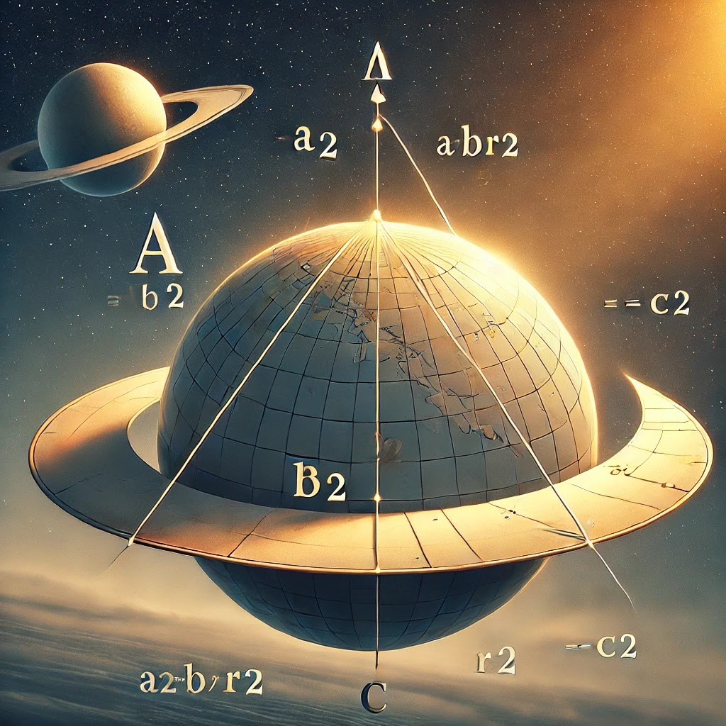
(File:Spherical triangle.svg - Wikipedia) A right-angled spherical triangle on a sphere. In spherical geometry (positive curvature), straight lines (geodesics) are great-circle arcs on the sphere. In the diagram, we see a right triangle on a sphere (dashed arcs along great circles). One angle is marked as 90°, forming a right triangle. In such a triangle, the sum of angles is more than 180° – in fact, the depicted triangle might have angles summing to about 270° (each corner here looks like ~90°). For this triangle, the sides $a, b, c$ (measured as arc lengths) violate the flat Pythagorean theorem: $a^2 + b^2$ will be larger than $c^2$. The curvature “pulls” the endpoints of the legs closer together than they would be in a plane, shortening the hypotenuse. This is why the formula uses a minus term for spherical space. If you tried to use Euclidean $a^2+b^2$ to predict $c$, you’d overestimate $c$. The red points in the diagram are the triangle’s vertices, and the dashed arcs illustrate the curved paths. Even though one angle is 90°, the side lengths do not satisfy $a^2+b^2=c^2$; instead, one finds $a^2+b^2 > c^2$. (For an extreme example, as noted, if each leg is 90° (¼ circumference), then $a = b = R\pi/2$ and one finds $c = R\pi/2$ as well, giving $a^2+b^2 = 2(R\pi/2)^2 = 2c^2$.)

(image) A right-angled hyperbolic triangle on a saddle surface. In hyperbolic geometry (negative curvature), lines “curve outward” and distances grow faster. The image shows a triangle drawn on a saddle-shaped surface (a surface of constant negative curvature can be locally represented by a saddle). The green region is a geodesic triangle on this saddle, and at least one angle (the one with the little square marker) is 90°. Notice how “spread out” the triangle appears – the saddle shape causes the triangle to occupy more area for given side lengths, and the third angle is visibly smaller than 90° (angle sum < 180°). In such a triangle, $a^2 + b^2$ is less than $c^2$. The space curves away, so the legs diverge more than they would on a plane, and the direct route (hypotenuse) is longer. Our formula’s $+ \frac{a^2 b^2}{R^2}$ term for hyperbolic geometry reflects this: you must add a positive amount to $a^2+b^2$ to get $c^2$. Equivalently, if you used $a^2+b^2$ naively, you’d under-estimate the true $c^2$. The saddle model is a physical visualization – mathematically, one often uses the Poincaré disk or half-plane model to draw hyperbolic triangles, but the saddle gives the right intuition of a space where geodesics deviate outward.

In both images, the curvature radius $R$ sets how pronounced these effects are. A sphere with larger radius (flatter sphere) would make the difference smaller; a saddle with a gentler curvature (larger $R$) likewise makes hyperbolic triangles closer to Euclidean. If one could shrink these triangles down to a tiny size, they would look almost flat – the 90° angle triangle on a very small patch of sphere or saddle would satisfy $c^2 \approx a^2+b^2$ closely. It’s only when the sides extend enough that the curvature accumulates that we see a strong deviation.

Applications and Interpretations

The curvature-corrected Pythagorean relationship has both conceptual and practical significance:

• Geometry and Topology: The failure of $a^2+b^2=c^2$ in curved space is a direct indicator of non-Euclidean geometry. In fact, as the Wikipedia entry notes, “were the Pythagorean theorem to fail for some right triangle, then the plane cannot be Euclidean” (Pythagorean theorem - Wikipedia). In differential geometry, one can show that the difference $a^2 + b^2 - c^2$ for an infinitesimal right triangle is proportional to the Gaussian curvature $K$. More precisely, for an infinitesimal right triangle one finds $c^2 = a^2 + b^2 - \frac{K}{3}a^2 b^2 + O(a^2 b^2)$. Our formula is a simplified finite-size extrapolation of this idea. This connects to Gauss’s Theorema Egregium – it tells us that curvature is an intrinsic property that affects distance relations. For finite triangles, the Gauss-Bonnet theorem relates the angle excess/defect (and thus indirectly the Pythagorean “error”) to the area and curvature: $a^2 + b^2 - c^2$ is tied to the area via $K$. Thus, the corrected theorem encapsulates a bit of the Gauss-Bonnet result in algebraic form.

• Law of Cosines generalization: As shown, the formula is essentially a low-order form of the spherical/hyperbolic law of cosines. In fact, one could present a general law of cosines with $h$ and $R$ that covers all cases: for a triangle with angle $C$ between sides $a$ and $b$, $\cos\!\frac{c}{R} = \cos\!\frac{a}{R}\cos\!\frac{b}{R} + h\,\sin\!\frac{a}{R}\sin\!\frac{b}{R}\cos C.$ Here plugging $C=90^\circ$ (so $\cos C=0$) yields the right-triangle versions above (with $\cos$ for $h=-1$ spherical and $\cosh$ implicitly for $h=+1$ hyperbolic by the change $\cos(ix)=\cosh(x)$). This unified view shows how $h$ enters to change the sign of the $\sin(a/R)\sin(b/R)$ term. The given $a^2 + b^2 + h\frac{a^2 b^2}{R^2} = c^2$ is essentially the small-angle (small side) expansion of this law. It’s a useful mnemonic and is sometimes used in approximate navigation or surveying calculations.

• Surveying and Navigation: Historically, surveyors over large distances had to account for Earth’s curvature. For instance, if you have two perpendicular straight paths on Earth of length $a$ and $b$, the straight-line distance (great circle) $c$ between the endpoints won’t exactly satisfy $a^2+b^2=c^2$. For moderate distances (say a few tens of kilometers), one could plug values into $a^2+b^2 - \frac{a^2 b^2}{R^2} = c^2$ with $R \approx 6371$ km (Earth’s radius) to get a correction. Usually, though, the effect is very small unless $a$ and $b$ are large – which is why for most local surveying, flat-Earth Pythagoras works fine. But for transcontinental distances, spherical trigonometry is mandatory. The formula gives a sense of the error: e.g. if $a = b = 100$ km, $a^2b^2/R^2 \approx (10^4 \text{ km}^2)^2/(6371^2 \text{ km}^2) \approx 2.46 \text{ km}^2$, so $a^2+b^2 = 2(10^4)^2 = 2\times10^8 \text{ m}^2$ versus $c^2 \approx 2\times10^8 - 2.46\times10^6 \text{ m}^2$, meaning $c \approx 141.27$ km instead of $141.42$ km flat – a difference of ~150 meters over 141 km, which is noticeable with precise measurement. Such corrections are relevant in geodesy (the science of measuring Earth).

• Astronomy and Cosmology: On the scale of the universe, space may be curved. Cosmologists speak of a “closed” universe (positive curvature), “open” universe (negative curvature), or flat universe. In principle, if we could construct a huge triangle between faraway galaxies or beams of light, the sum of angles or the relation between lengths would diagnose cosmic curvature. The equation $a^2 + b^2 + h \frac{a^2 b^2}{R^2} = c^2$ can be seen as a clue: if the universe had curvature radius $R$ not extremely large, very large right triangles would show a deviation. So far, observations (e.g. of the cosmic microwave background’s angular-size fluctuations) indicate that if there is any curvature, $R$ is extremely large (on the order of the observable universe or more), meaning the correction term is essentially zero for any triangle we could observe – in other words, space appears nearly flat on the largest scales.

• General Relativity: In GR, local space can be curved by mass. However, most curvature in GR is in 4D spacetime and involves time, so a spatial triangle in a static gravitational field might show a tiny effect, but it’s subtle (GR would more directly affect the sum of angles through spacetime geometry rather than a pure space-distance Pythagorean relation, unless one measures spatial geodesics around a mass). Nonetheless, conceptually, the fact that $a^2+b^2=c^2$ can fail in a gravitational field is related to spatial curvature produced by mass. For example, around a massive object, space is slightly curved (positive curvature in the Schwarzschild spatial geometry outside a mass), so a large triangle around a star could have an angle excess and a corresponding Pythagorean deficit. Such effects are usually quite small except in strong gravity. Experiments to detect spatial curvature on small scales are challenging – one interesting tabletop test by J. Martinis (2012) actually tried to detect a deviation from $a^2+b^2=c^2$ by constructing physical right triangles out of metal plates and weighing the areas () (). The result was null within experimental error, as expected – any curvature of space caused by local mass was far too tiny (they set a lower bound on an effective $R > 2.2$ m for space curvature in their lab () (), whereas Earth’s actual curvature radius is much larger and GR curvature caused by Earth’s gravity is larger still but still not observable at that scale).

• Education and Intuition: The corrected formula is pedagogically useful. It provides a gentle introduction to non-Euclidean geometry by modifying a familiar equation. Students can plug in numbers to see, for instance, that on a sphere of radius $R$, a right triangle with legs of significant length shows a noticeable difference. It bridges algebra and geometry: one can calculate with it, not just qualitatively say “angles sum to > 180°.” For hyperbolic geometry, which is harder to visualize, the formula gives a quantitative handle: if $R=1$ (unit curvature) and $a=b=1$, then $a^2+b^2+c^2$ would imply $c = \sqrt{1+1+1} = \sqrt{3} \approx 1.732$, whereas flat would give $c=\sqrt{2}\approx1.414$. Indeed, rigorous hyperbolic trig would yield $\cosh c = \cosh 1 \cosh 1$, from which $c \approx 1.527$ (smaller than $\sqrt{3}$ because our formula’s coefficient should be 1/2 for small sides), but the trend is correct that $c$ is bigger than 1.414. This kind of numerical exploration builds intuition about how triangles work in these exotic geometries.

In conclusion, the “Pythagorean” curvature-correction formula $a^2 + b^2 + h\,\frac{a^2 b^2}{R^2} = c^2$ is a compact way to express the leading influence of curvature on distance relationships. Chirality is encoded by $h=±1$, distinguishing the “handedness” of space (positively or negatively curved). The signs of the terms indicate whether the geometry makes the hypotenuse shorter or longer than Euclid’s prediction. The radius $R$ quantifies how significant the deviation is – with flat space as the infinite-radius limit. The formula is grounded in the curved-space Law of Cosines and provides an approachable approximation to it. Whether for computing long-distance paths on Earth, conceptualizing cosmic geometry, or simply understanding the link between algebra and geometry in curved spaces, this corrected Pythagorean theorem is a powerful illustrative tool. As Gauss and Bolyai discovered, and as the above analysis shows, Euclidean Pythagoras is a special case – in a world with curvature, a little extra (or a little less) is needed to close the triangle (Pythagorean theorem - Wikipedia).